Mantid#
Mantid (https://mantidproject.org/) serves as one of the main tools for reducing and interacting with single crystal diffraction data.
Mantid Workbench#
Workbench is the graphical user interface for Mantid. Opening Workbench, the first page presented is a splash screen for selecting a facility and instrument. This step is optional, but it may be desirable as some shortcut presets are automatically filled in to reflect the chosen instrument.
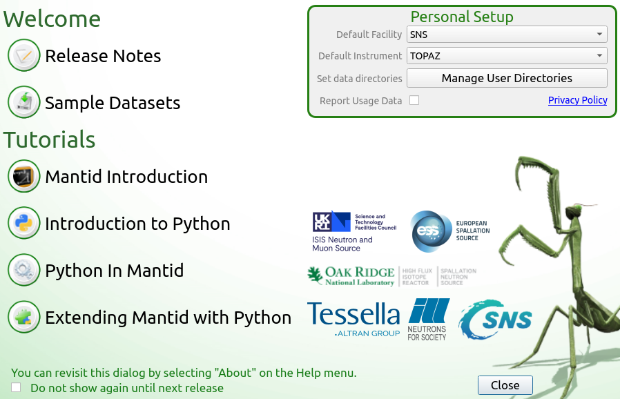
Selecting a default facility (SNS/HFIR) and instrument (TOPAZ/MANDI/CORELLI/SNAP/DEMAND/WAND²).#
There is a option to skip this splash screen the next time Workbench is opened. Click this before closing the screen in order to save as default.
Main page#
The main page provides several areas to navigate. Among them are:
Workspaces (upper left): viewing data
Algorithms/Plots (lower left): running a data processing step or viewing a previous plot
Editor/IPython (central): running a script or performing calculations
Messages (right): console messages including errors, intermediate results, and status
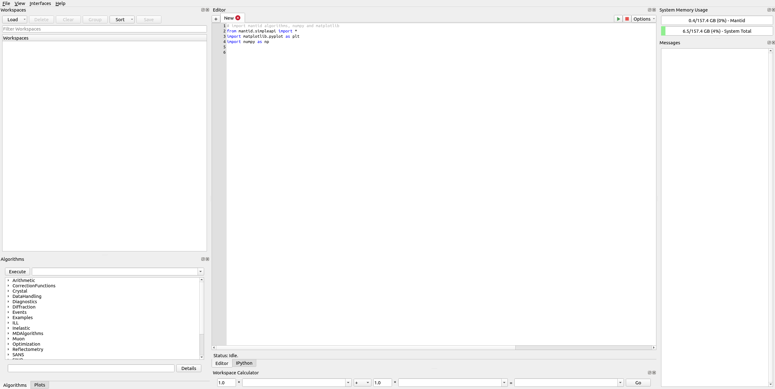
Mantid Workbench.#
The workspaces area contains a list of all workspaces currently in memory. The dropdown below each name contains information about the workspace including its type.
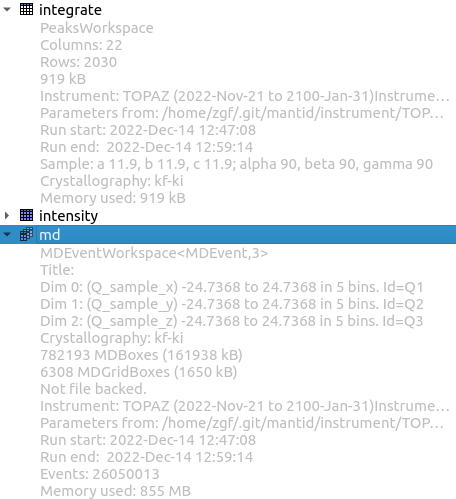
Workspaces.#
A right-click can be used to bring up options for interacting with the data. The options available depend on the workspace type. Some examples include:
Show Data
Rename
Save Nexus
Delete
Higlighting a workspace, an algorithm can be run on it by typing an algorithm name. The name can be searched either by typing or chooising from categories.
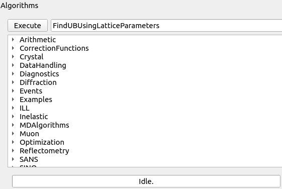
Algorithms.#
The progress bar of a running algorithm is shown. Idle indicates that no algorithm is currently being run. The Details button can be clicked to view additional details and even Cancel a running one. The plot area contains previously created plots that can be reopened.

Plots.#
A console for performing basic calculations or interacting with the workspaces is available.

IPython console.#
Use mtd.importAll() to make all the workspaces available with handles based on the workspace name.
Note
It is advisable to monitor system and session usage. If more memory is needed, consider using a different resource node.

Session and system memory usage.#
Running a script#
The following example demonstrates some basic processing of single crystal data in Workbench.
Load data
Transform to reciprocal space
Find strong peaks
Find initial UB
Predict peaks
Integrate peaks
Code can be executed in the editor.

Mantid Workbench editor.#
Three main imports are typically used.
Mantid algorithms for data interaction
matplotlib pyplot interface for plotting
numpy for basic numerical/array calculations
Once a script is loaded or written, it can be run by pressing the play button. The script can also be stopped with the stop button.

Script editor play/stop buttons.#
 """
 This script demonstrates the workflow for TOPAZ data reduction using Mantid.
 It includes steps to find the UB matrix of a single crystal sample, index,
 and integrate peaks for a single run.

 Workflow:
 1. Load and preprocess data.
 2. Set sample and lattice parameters.
 3. Convert data to multidimensional workspace.
 4. Find and index peaks.
 5. Integrate peaks.
 6. Create MDHisto HKL Workspace
 7. Save Results
 """

 # Import necessary libraries and Mantid algorithms
 import os
 from mantid.simpleapi import *
 from mantid import config
 import matplotlib.pyplot as plt
 import numpy as np

 # Set the Q convention to 'Crystallography'
 config["Q.convention"] = "Crystallography"

 ### Experiment data information ###
 IPTS = 33715
 run = 46917

 # Base name for the TOPAZ experiment
 exp_name = "garnet"

 output_directory = f"/SNS/TOPAZ/IPTS-{IPTS}/shared/CrystalPlan"

 ### Sample information ###
 a, b, c = 11.93, 11.93, 11.93
 alpha, beta, gamma = 90, 90, 90
 cell_type = "Cubic"
 centering = "I"

 ### Incident wavelength range ###
 wavelength_band = [0.5, 3.5]

 ### Peak finding parameters ###
 max_peaks = 500
 strong_threshold = 100

 ### Peak indexing tolerance ###
 tol = 0.1

 ### Peak integration radius ###
 r_cut = 0.2

 # Check if the directory exists, and create it if it doesn't
 if not os.path.exists(output_directory):
     os.makedirs(output_directory)
 print(output_directory)

 # Set the working directory
 os.chdir(output_directory)

 # Create a single valued workspace to hold sample data
 CreateSingleValuedWorkspace(OutputWorkspace="sample")

 # Set the Unit Cell parameters for the sample
 SetUB(Workspace="sample", a=a, b=b, c=c, alpha=alpha, beta=beta, gamma=gamma)

 # Get lattice parameters
 lattice = mtd["sample"].sample().getOrientedLattice()
 astar, bstar, cstar = lattice.astar(), lattice.bstar(), lattice.cstar()

 # Calculate Q_min and d_max
 Q_min = 2 * np.pi * min([astar, bstar, cstar])
 d_max = 2 * np.pi / Q_min

 # Unpack wavelength range
 wl_min, wl_max = wavelength_band

 # Define reflection condition dictionary
 refl_cond_dict = {
     "P": "Primitive",
     "I": "Body centred",
     "F": "All-face centred",
     "R": "Primitive",  # rhombohedral axes
     "R(obv)": "Rhombohderally centred, obverse",  # hexagonal axes
     "R(rev)": "Rhombohderally centred, reverse",  # hexagonal axes
     "A": "A-face centred",
     "B": "B-face centred",
     "C": "C-face centred",
 }

 # Load the data file
 filename = f"/SNS/TOPAZ/IPTS-{IPTS}/nexus/TOPAZ_{run}.nxs.h5"
 LoadEventNexus(Filename=filename, OutputWorkspace="data")

 # Set the goniometer settings
 SetGoniometer(
     Workspace="data",
     Axis0="BL12:Mot:omega,0,1,0,1",
     Axis1="BL12:Mot:chi,0,0,1,1",
     Axis2="BL12:Mot:phi,0,1,0,1",
     Average=True,
 )

 omega = mtd["data"].getRun()["omega"].value[0]
 print("Goniometer Omega = {: 8.3f}".format(omega))

 # Preprocess detectors
 PreprocessDetectorsToMD(InputWorkspace="data", OutputWorkspace="detectors")

 # Calculate Q_max and d_min
 two_theta = mtd["detectors"].column("TwoTheta")
 Q_max = 4 * np.pi / wl_min * np.sin(0.5 * max(two_theta))
 d_min = 2 * np.pi / Q_max

 # Convert data to MD workspace
 ConvertToMD(
     InputWorkspace="data",
     QDimensions="Q3D",
     dEAnalysisMode="Elastic",
     Q3DFrames="Q_sample",
     LorentzCorrection=True,
     MinValues=[-Q_max, -Q_max, -Q_max],
     MaxValues=[+Q_max, +Q_max, +Q_max],
     PreprocDetectorsWS="detectors",
     OutputWorkspace="md",
 )

 # Find peaks in the MD workspace
 FindPeaksMD(
     InputWorkspace="md",
     MaxPeaks=max_peaks,
     PeakDistanceThreshold=Q_min,
     DensityThresholdFactor=strong_threshold,
     OutputWorkspace="strong",
 )

 # Index the peaks using the lattice parameters
 FindUBUsingLatticeParameters(
     PeaksWorkspace="strong",
     a=a,
     b=b,
     c=c,
     alpha=alpha,
     beta=beta,
     gamma=gamma,
     Tolerance=tol,
 )

 # Index the found peaks
 IndexPeaks(PeaksWorkspace="strong", Tolerance=tol, RoundHKLs=True)

 # Filter peaks based on h^2 + k^2 + l^2 > 0
 FilterPeaks(
     InputWorkspace="strong",
     OutputWorkspace="strong",
     FilterVariable="h^2+k^2+l^2",
     FilterValue=0,
     Operator=">",
 )

 # Calculate peak intensity vs radius
 PeakIntensityVsRadius(
     InputWorkspace="md",
     PeaksWorkspace="strong",
     RadiusEnd=r_cut,
     NumSteps=51,
     BackgroundInnerFactor=1,
     BackgroundOuterFactor=1.5,
     OutputWorkspace="intensity",
     OutputWorkspace2="signal-to-noise",
 )

 # Extract the number of peaks from the signal-to-noise workspace
 ExtractSingleSpectrum(
     InputWorkspace="signal-to-noise",
     OutputWorkspace="number-of-peaks",
     WorkspaceIndex=0,
 )

 # Estimate fit parameters for the peak intensity
 A = mtd["number-of-peaks"].extractY().max()
 constraints = ",constraints=(0<A<{},0<sigma<{})".format(2 * A, r_cut / 6)
 function = "name=UserFunction,Formula=A*(erf(x/(sqrt(2)*sigma))-sqrt(0.5/atan(1))*(x/sigma)*exp(-0.5*(x/sigma)^2))"
 EstimateFitParameters(
     Function=function + constraints,
     InputWorkspace="number-of-peaks",
     IgnoreInvalidData=True,
     OutputWorkspace="params",
 )

 # Extract peak and background radii
 I, sigma = mtd["params"].column(1)
 peak_radius = 3 * sigma
 delta = 0.01
 bkg_inner_radius = (1 + delta) * peak_radius
 bkg_outer_radius = ((2.15 + delta) ** (1 / 3)) * peak_radius
 ellipse_region_radius = 1.2 * bkg_outer_radius

 integrate_if_edge_peak = True  # for sphere integration only

 # Print the calculated radii
 print(f"Peak radius {peak_radius:5.3f}")
 print(
     f"Peak inner, outer and region radii {bkg_inner_radius:5.3f}, {bkg_outer_radius:5.3f}, {ellipse_region_radius:5.3f}"
 )

 # Predict peaks based on the UB matrix
 PredictPeaks(
     InputWorkspace="strong",
     WavelengthMin=wl_min,
     WavelengthMax=wl_max,
     MinDSpacing=d_min,
     MaxDSpacing=d_max,
     ReflectionCondition=refl_cond_dict[centering],
     EdgePixels=18,
     OutputWorkspace="peaks",
 )

 # Integrate peaks using ellipsoids
 IntegrateEllipsoids(
     InputWorkspace="data",
     PeaksWorkspace="peaks",
     RegionRadius=ellipse_region_radius,
     SpecifySize=True,
     PeakSize=peak_radius,
     BackgroundInnerSize=bkg_inner_radius,
     BackgroundOuterSize=bkg_outer_radius,
     OutputWorkspace="peaks",
     CutoffIsigI=5,
     AdaptiveQBackground=True,
     AdaptiveQMultiplier=0.001,
     UseOnePercentBackgroundCorrection=False,
 )

 # Filter peaks based on signal-to-noise ratio
 FilterPeaks(
     InputWorkspace="peaks",
     OutputWorkspace="peaks",
     FilterVariable="Signal/Noise",
     FilterValue=3,
     Operator=">",
 )

 IndexPeaks(
     PeaksWorkspace="peaks",
     Tolerance=0.10,
     ToleranceForSatellite=0.10,
     RoundHKLs=False,
     CommonUBForAll=True,
 )

 # Repeat integration after filtering
 IntegrateEllipsoids(
     InputWorkspace="data",
     PeaksWorkspace="peaks",
     RegionRadius=ellipse_region_radius,
     SpecifySize=True,
     PeakSize=peak_radius,
     BackgroundInnerSize=bkg_inner_radius,
     BackgroundOuterSize=bkg_outer_radius,
     OutputWorkspace="integrate",
     CutoffIsigI=5,
     AdaptiveQBackground=True,
     AdaptiveQMultiplier=0.001,
     UseOnePercentBackgroundCorrection=False,
 )

 # Final filtering of peaks
 FilterPeaks(
     InputWorkspace="integrate",
     OutputWorkspace="integrate",
     FilterVariable="Signal/Noise",
     FilterValue=3,
     Operator=">",
 )

 OptimizeLatticeForCellType(
     PeaksWorkspace="integrate",
     CellType=cell_type,
     Apply=True,
     Tolerance=0.1,
     EdgePixels=18,
     OutputDirectory="./",
 )

 # Calculate maximum h, k, l based on Q_max
 max_h, max_k, max_l = np.floor(
     Q_max / (2 * np.pi * np.array([astar, bstar, cstar]))
 )

 # Convert Q to HKL in MD histogram
 ConvertQtoHKLMDHisto(
     InputWorkspace="md",
     PeaksWorkspace="peaks",
     UProj=[1, 0, 0],
     VProj=[0, 1, 0],
     WProj=[0, 0, 1],
     Extents=[-max_h, max_h, -max_k, max_k, -max_l, max_l],
     Bins=[301, 301, 301],
     OutputWorkspace="hkl",
 )

 # Copy sample data to the HKL workspace
 CopySample(
     InputWorkspace="peaks",
     OutputWorkspace="hkl",
     CopyName=False,
     CopyMaterial=False,
     CopyEnvironment=False,
     CopyShape=False,
 )

 SaveIsawPeaks(
     InputWorkspace="integrate",
     Filename=output_directory + exp_name + "_" + str(run) + ".integrate",
     RenumberPeaks=True,
 )
 SaveIsawUB(
     InputWorkspace="integrate",
     Filename=output_directory + exp_name + "_" + str(run) + ".mat",
 )
 SaveMD(
     InputWorkspace="hkl",
     Filename=output_directory + exp_name + "_" + str(run) + "_hkl.md",
 )
After running the script, the steps can be investigated.
Instrument viewer#
For event data, an instrument view is available for investigating the data in detector-space. This is done by navigating to the workspace area:
Right-click data
Left-click Show Instrument
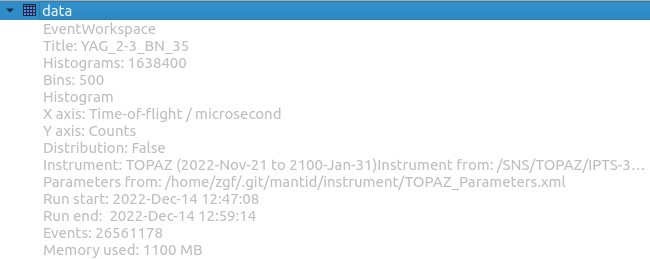
Event data workspace.#
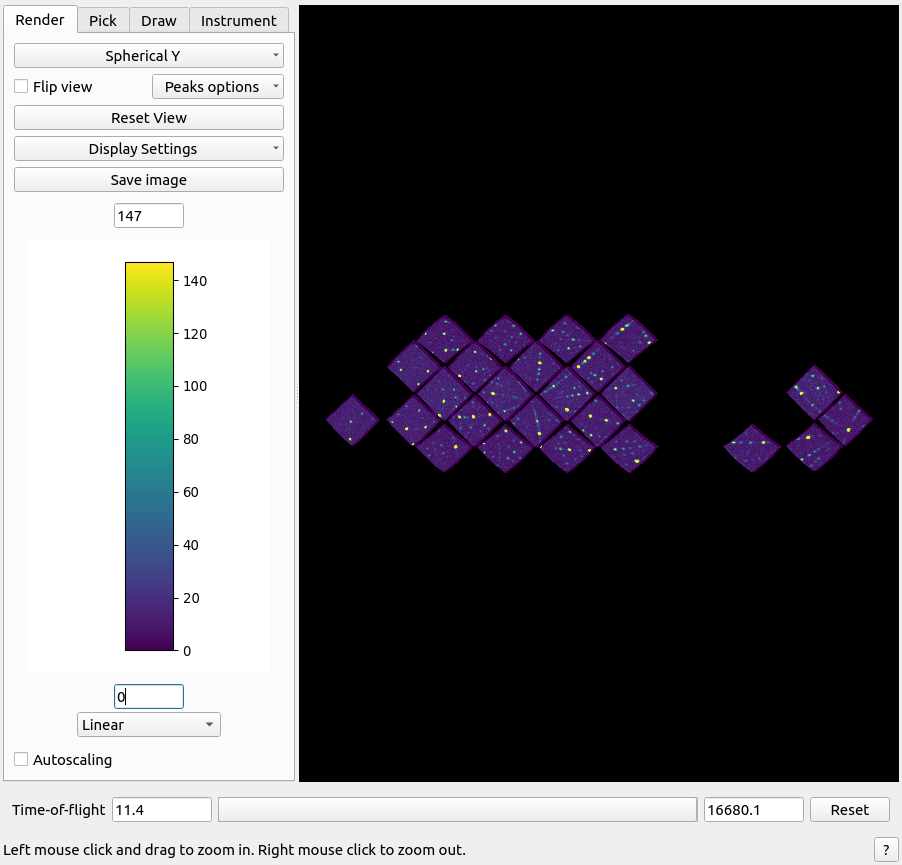
Instrument viewer.#
It is possible to change the view, zoom in and out, and highlight regions of interest.
Plot viewer#
Certain workspaces can be viewed as a plot.
Right-click signal-to-noise
Right-clicl Plot>`Spectrum`
Right-click Plot All
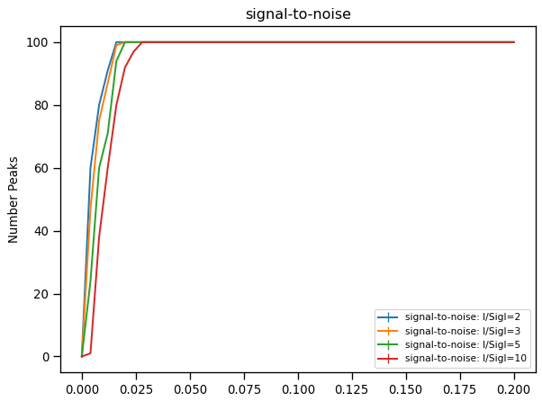
Plot.#
It is possible to change the look of the plot and save it to a file. Other options include the capability to fit the data or generate a script to generate the plot through the editor.

Plot tool bar.#
Slice viewer#
The slice viewer is a valuable tool for investigating three-dimensional data like reciprocal space data. This includes rebinnable 3d-event workspaces and 3d-histogram workspaces. Slice viewer for a workspace can be opened from the workspace area:
Right-click md
Left-click Show Slice Viewer
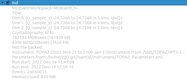
Event data workspace.#
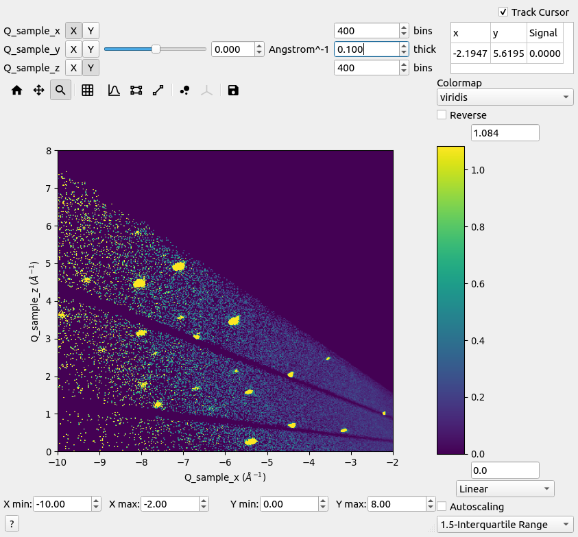
Slice viewer.#
Slice viewer allows data to be displayed in various ways. For 3d data, the display axes X (horizontal) and Y (vertical) directions can be chosen. The remaining axis can be sliced where its level is chosen from the slider.

Display axis and slider value shown of a typical x0z-slice for Q-sample data.#
For rebinnable reciprocal space data, there are also options for changing the bin number and slice integration thickness. This is not possible for histogram data. The axes limits can be adjusted, if needed.

Display axis zoom limits.#
It is also possible to zoom by holding a left-click a rectangular region-of-interest. The color bar can also be changed. This includes the color map, normalization and scaling limits that may be adjusted manually or automatically.

Colorbar parameters.#
For automatic autoscaling, there are 3 options for selecting the limits that include.
Min/Max: adjust to minimum and maximum values of the data
3-sigma: adjust to three standard deviations below and above the mean of the data
1.5-Interquartile Range: adjust interval to below the first quartile and above the third quartile beyond 1.5 times the interquartile range of the data
1.5-Median Absolute Deviation: adjust interval to below and above the median using 1.5 times the median absolute deviation of the data
It is also possible to change the normalization. Options include:
Linear: linear scaling
Log: logarithmic scaling (valid for positive values only)
SymmetricLog10: symmetric logarithmic scaling but linear near zero
Power: power scaling
There is a capability to track the coordinate and value of the cursor. By unchecking Track Cursor, a left-click on the map can be used to select a coordinate individually.
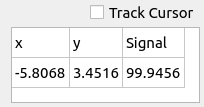
Cursor position and value.#
There is a main tool bar with several options.
Home
Pan
Zoom
Grid lines
Line plots
Region selection
Line cut
Peaks overlay
Non-orthogonal stretch (hkl-like axes, only)
Save image

Tool bar options.#
Choose the peaks option to overlay peaks to view the peak positions and/or integration regions.
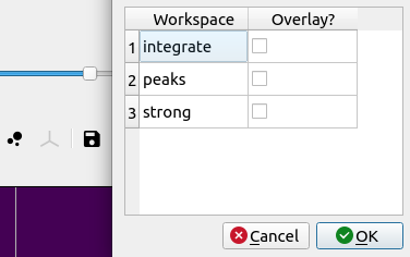
Choose peaks to overlay.#
Click on a row to highlight a peak and automatically zoom to the region near the peak.
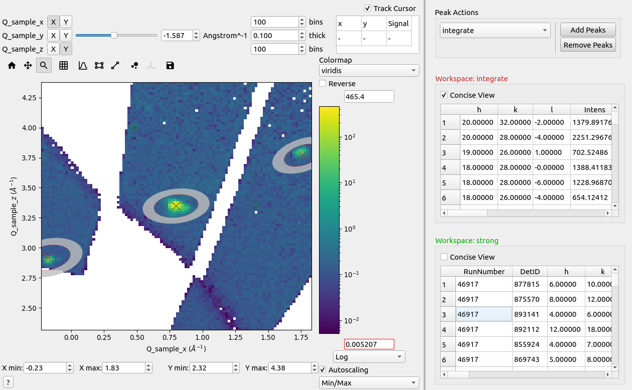
Peaks in reciprocal space.#
A binned histogram workspace can also be viewed.
Right-click hkl
Left-click Show Slice Viewer
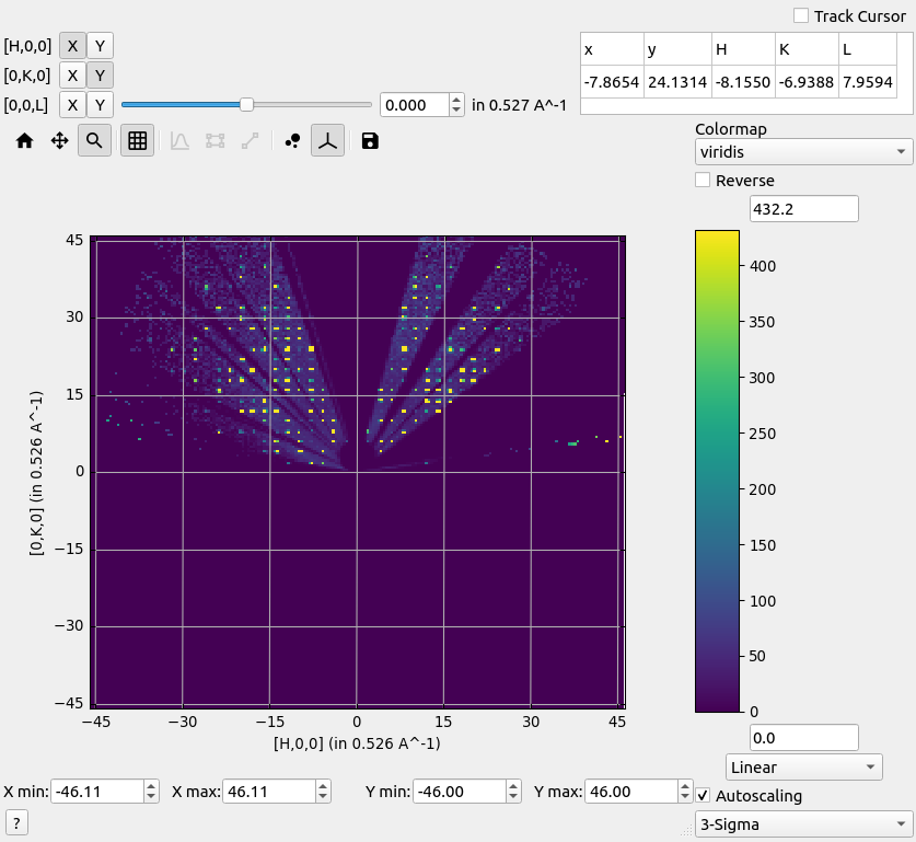
Reciprocal space hkl-map.#
Choose the non-orthogonal option to stretch the axes according to the reciprocal lattice parameters.
Peaks table viewer#
A peaks workspace can be viewed with all details listed in a table by right-clicking on the workspace and choosing Show Data. The peaks viewer represents each peak as a row and different attributes about them as a column. These are the columns:
RunNumber: Run number
DetID: Detector (pixel) ID
h: h-index
k: k-index
l: l-index
Wavelength: Wavelength
Energy: Energy
TOF: Time-of-flight
DSpacing: d-spacing
Intens: Integrated intensity
SigInt: Integrated intensity uncertainty
Intens/SigInt: Signal-to-noise raio
BinCount: Bin count
BankName: Bank name
Row: Pixel row
Col: Pixel column
QLab: Q-laboratory vector
QSample: Q-sample vector
PeakNumber: Peak number
TBar: Absorption weighted path length
IntHKL: Integer hkl vector
IntMNP: Integer mnp vector

Peaks table viewer.#

